
Traditional indexing works extremely well for traditional data. Spatial data, however, does not fit the expected model of trafditional data that RDBMSs like to use.
There are three general spatial data types that are typically used to represent geographic reality. We will focus on two dimensional types. The three types are: point, line, and region. Furthermore, they are differentiated into two classes: simple and complex.
Definition: Simple point, line, and region
A simple point is a single point in euclidean space: (x,y)
A simple line is a connected, one dimensional object in euclidean space with two end points.
A simple region is a single, simple, minimal cycle separating the interior of the region from the exterior of the region (A Jordan curve)

Definition: Complex point, line, and region
A complex point, sometimes called a multi-point, is a collection of non-overlapping, simple points
A complex line is a collection of disjoint simple lines
A complex region is a collection of faces and holes. A face is a simple region, possibly containing holes. A hole fits the definition of a simple region, but the interior of a region lies on the exterior of a hole, and the exterior of a region lies on the interior of a hole. Faces can contain multiple holes, and multiple faces can occur within a hole. Faces and holes can touch along their boundaries at a finite number of discrete points.

In mathematical terms, all data types are considered to be regular open point sets. This has desirable properties for the semantics of operations. All spatial objects have three components: an interior, and exterior, and a boundary.
Why are simple data types not sufficient? (think in terms of geographic reality, operations that must be performed, and object oriented conceptualization).
The mathematical definitions of spatial types are based on point set topology. Types are defined by using infinite point sets, not directly representable in computers.
So, we discretize them by storing their boundaries. Furthermore, boundaries are stored as straight line segments. Straight line segments are easy, they have easy geometry, they require no computation to generate, and they are accurate enough.
So... how many straight line segments does it take to represent Texas, Louisiana, Arkansa? Should we shoot for compact representations, or more detailed representation. what about portions of boundaries that are straight? Take a look at the TIGER data ( The image below is published by the US. Census Bureau at http://www.census.gov/geo/maps-data/maps/reference-cd113.html ) ...

Databases love fixed size records. How do we incorporate spatial data
Concept: Spatial Data In RDBMS
RDBMSs like fixed sized records, in fact, many traditional index structures rely on this.
Solution: In a table, create a column of a geometry type. The record simply contains a pointer (disk address) of the actual geometry. 1 level of indirection.
Counties (Name string(30), stateAbbrv string(2), population int, geometry region)
Now, records get to use the existing index structures, but we have the ability to add new index types for the spatial data.
When considering index structures, it make sense to consider the types of queries that will access them. Recall the B+ tree’s ability to link adjacent leaf nodes supporting range queries. For point data, there are lots of possible types of queries, here are some common ones:
 nearest neighbors to a query point. The value of can be 1 to find the nearest neighbor, in which cas it is just a nearest neighbor query.
What are some examples of real world applications that use these query types? Consider ecology, biology, mapping, climatology, anything else you can think of.
We typically know something about the data. For example, how much to expect, roughly where it will be, some kinds of bounds.
Simplist way to index space just break it up into a uniform grid.

Computational based. We don’t have to store the grid cells. For a universe from 0-10 in X and Y direction, and 10 cells in each dimension, what cell does the point  lie in?
 where
 .
Where do we store the actual points (remember our disk page behavior)? Each grid cell must point to a disk page where the points in that cell are stored. If a page fills up, we simply chain them, much like the leaves of a B+tree.
So, we need an index file that translates grid cells to disk pages.
Queries
What is the procedure to compute a nearest neighbor query for the point  ? In the BEST case, how many disk pages do we read? In the worst case, how many disk pages do we read? How many times do we query the index file? Repeat the question for
 .
What is the procedure to compute a range query: “Find all points in the rectangle defined by  . Best case disk page reads? worst case disk page reads?
What is the procedure to find all points in within a radius of 2 from ? Best case disk page reads? worst case disk page reads?
One problem for grid files, the disk pages for each cell are not necessarily stored near each other on disk!
Advantages:
Disadvantages:
 space in the index file. Possibly list in the index file that the cell is empty. Possibly use a hash table approach.
Clearly, 2 adjacent grid cells in a grid index cannot always be adjacent on disk (a cell has 8 neighbors!). How do we arrange cells on disk to improve seek time and reduce effective rotational latency? Instead of random cell placement on disk, follow some kind of ordering.
Z ordering is a method of mapping 2 (or higher) dimensions to a lower dimensional ordering (typically 1). We want a two dimensional cell structure to map to a 1 dimensional disk addressing scheme such that cell neighbors tend to end up close to each other on disk.
Z ordering works by interleaving the bit representations of a cell address:

If we interleave the bits of each cell address, we end up with a linear ordering of the cells. You can see where the Z ordering gets its name:

For example, the cells (0,0), (0,1), (1,0), (1,1) get the following interleaved bit addresses (red bit goes first and are numbers, green bits are o and t):
0 o 0 o 0 o 0 o: (0,0) = 0
0 o 0 o 0 o 0 t: (0,1) = 1
0 o 0 o 0 o 1 o: (1,0) = 2
0 o 0 o 0 o 1 t: (1,1) = 3
0 o 1 o 0 t 1 o: (2,5) = 38
0 o 1 o 0 t 1 t: (3,5) = 39
Queries:
What is the procedure to compute a nearest neighbor query for the point  ? In the BEST case, how many disk pages do we read? In the worst case, how many disk pages do we read? How many times do we query the index file?
What is the procedure to compute a range query: “Find all points in the rectangle defined by . Best case disk page reads? worst case disk page reads?
What is the procedure to find all points in within a radius of 2 from  ? Best case disk page reads? worst case disk page reads?
So... why is the z-ordering superior to the straight grid file? Spatial Proximity
The problem with grid based stuctures is that they are static! They do not adapt effectively to the input. In other words, they are highly sensitive to data skew, in which a lot of the data might exist in a small area of the grid. If the data is evenly distributed, grids work well.
The k-d tree is an adaptive data structure that will adjust to fit the data. It is a binary tree in which every node represents a point in one of k dimensions. Non leaf nodes effectively divide a hyperplane into two half-spaces (two parts). Each level in the tree typically cycles among which axis the hyperplane will be perpendicular to. Items that are left of the hyperplane will go into a left subtree, items right of a hyperplane will go in a right subtree.
Construction of the tree is as follows:
Example
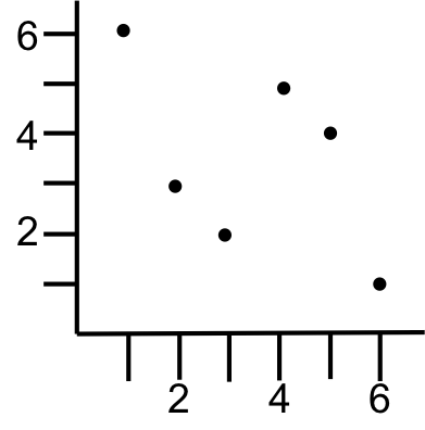
Lets build a k-d tree with the points: (1,6), (2,3), (3,2) (4,5), (5,4), (6,1). We will start splitting on the x dimension.
A split will stop when it enocounters a previosly existing split line.
Root node: split on x axis at median of x values = 4: (4,5)
left subtree will have: (1,6), (2,3), (3,2)
split on y axis at median of y values: 3: (2,3)
left subtree will have: (3,2) – make final split on x axis
right subtree will have: (1,6) – make final split on y axis
right subtee will have: (5,4), (6,1)
split on y axis of median of y values 4: (5,4 )
left subtree will have: (6,1) – make final split on x axis


Note that the X levels in the tree act like the oprdering of a binary search tree, as do the Y levels. This property allows us to discover the rectangular subdivision of space implied by the tree rather easily. For example, to find the rectangle contianing the point (3.5,3.5), we simply follow the tree like a binary search tree, keeping track of the relevant extrema values:
Therefore, the contianing rectangle ranges are 1 to 4 in the x direction, and 3 to +infinity in the y direction
Inserting: Inserting follows the same binary search tree procedure to identify the insertion point. Insertions occur at leaves.
Deleting: find the node to delete, and then rebuild the tree consisting of all children of that node. OR, do a binary search tree style delete
Properties
Using the tree creation algorithm, a K-d tree is balanced (we always choose the median value). Inserts and deletes may cause the tree to become unbalanced. Thus, it is not a self-balancing search tree.
Time complexity of building the tree:
 input points. input points.
 times because it forms a balanced binary tree.
Because $k$ is an input parameter, it affects the number of comparisons to splitting planes.
Final time complexity is  for building the tree.
The basic k-d tree cannot be re-balanced, but adaptive k-d trees do exist.
Basic approach to the nearest neighbor:
Example
Find the nearest neighbor in the above tree to (4.1, 2)
Search the tree to identify node (6,1) with distance = 
back up to (5,4) with distance = 1.7 ((6,1) is still closest),  , so no need to search the right child of (5,4)
back up to (4,5) with distance = 2.9 ((6,1) is still closes),  , so we need to search the left child of (4,5)
recursively search. Find the insert point as a child of (3,2). with distance = 1.05 closest!
back up to (2,3) with distance = 1.8 ((3,2) is still closest).  , so we need to check right child of (2,3)
find (1,6), which is farther than 1.05, so back up the tree
already checked both sides of (2,3)
already checked both sides of (4,5)
Quad trees are another popular alternative to the fixed spatial decomposition scheme of grid files. Quad trees recursively divide space into quadrants until each quadrant contains a maximum number of elements. The maximum number of elements is a decision made before the quad tree is constructed, and will often depend on a disk page size. In essence, the maximum number of elements in a quadrant should be manageable based on some designe constraint.
Let  be the maximum number of elements grouped together into a leaf node of a quad tree for point data.
The basic idea is to begin with the entire embedding space, and see if the are more than elements. If so, then the space is divided into 4 equal quadrants. A root node is created, and leaf nodes, one per quadrant, are attached. Points in each quadrant are recorded in the corresponding leaf node. The procedure is applied recursively to each leaf node. If a leaf node contains fewer then points, the we do not subdivide the node..
Example
Create a quad tree using the following data set..

Compare the spatial decomposition to that of the uniform grid:
Avantages:
Disadvantages:
Queries
What is the procedure to compute a nearest neighbor query for the point ? In the BEST case, how many disk pages do we read? In the worst case, how many disk pages do we read? How many times do we query the index file? Repeat the question for .
What is the procedure to compute a range query: “Find all points in the rectangle defined by . Best case disk page reads? worst case disk page reads?
What is the procedure to find all points in within a radius of 2 from ? Best case disk page reads? worst case disk page reads?
Quad trees intuitive, they are adaptable to the data distribution, and they provide simple query constructions, but they do not generalize to a disk based structure very effectively. R-trees are the answer to that drawback of quad trees. The idea of an R-tree is to generalize a B-tree to handle two (or multi-) dimensional data.
The first problem we run into is that the problem of dimensionality with spatial data. B-trees rely on a total ordering or integers that corresponds to physical nearness across the dimensionality of the data (one dimensional integers). Points, are two dimensional. We can define a total ordering of points, but two points that are adjacent in ordering are not necessarily physically near to each other. The ordering does not imply physical nearness.
Exercise
Define a total ordering over points. Draw three points where two points that adjacent in the ordering are not the nearest points in the embedding space. Do the same with regions.
The idea of the R-tree is that physically near objects are grouped together in nodes in the R-tree. Like a B-tree, actual objects are stored only at leafs, and internal nodes provide a search path to the appropriate leaves. R-trees are balanced, have a fixed node size, and have constraints as to the minimum amount of objects allowed in a node. In essence, R-trees are similar in concept to B-trees, but with modifications to handle multi-dimensional data.
The main problem with R-trees is making sure that internal nodes don’t overlap too much, internal nodes don’t contain too much empty space, and that objects that are close together in space are actually stored close together in the tree.
An internal tree node will contain minimum bounding rectangles (MBRs). Associated with each MBR is a single pointer to a node such that the MBR minimally encloses all spatial objects in that node. (Note the single pointer, as opposed to a data element separating two pointers in a B-tree). When a node is full, it is split, objects are assigned to new nodes, and the MBRs of each node are adjusted. A MBR is then promoted (like a B-tree) to the parent node. A split can propogate all the way to the root, possibly growing the tree by one level.
Example
In this example, we will build up the R tree by adding a single regions at a time. Assume an R-tree that holds at most 3 object pointers per node. Adding regions to the root node is straightforward, and behaves much like a B tree.

Adding the fourth region requires a split. We must choose which regions to group together. Ideally regions near each other will be grouped together.

To insert the 5th region, we must choose which bounding rectangle to expand. Again, we want to use some heuristic, such as the expansion that covers the least additional area.

Adding the 6th region requires another split, and the root node is now full. We go ahead and add the 7th region since it does not force a split

Finally, the eight node will force a split, and the promoted bounding rectangle will also force a split, causing a split all the way up to the root

An alternative, and better, choice of bounding rectangles when inserting the 8th region. Why is it better?

Note that algorithms exist to efficiently build an R tree from a set of input regions. Such algortihms can have much better performance than continously inserting regions one by one because they avoid node splitting and tree growing, resulting in fewer disk I/Os.
Queries
What is the procedure to compute a nearest neighbor to region 1? In the how many disk pages do we read? Repeat for Region 7.
What is the procedure to compute a range query: “Find all points in the rectangle defined by an MBR surrounding regions 7,3, and 5? How many disk page reads?
Advantages:
Disadvantages:
Various heuristics can be used to choose which spatial objects to group together in a node. They generally involve tradeoffs in proximity/ empty space coverage/ thinness of MBRS.
R-trees are supported in virtually all commercial spatial databases. Lots of approaches have been developed to get around the problem of degenerate R-trees: multiple R-trees designed around the particular application (drones taking hi-resolution images), using the boundary line segments as the objects being stored instead of the entire regions, etc.
Variants: R*tree (different splitting and MBR choosing criteria, R+tree)