Big Data

This module discusses approaches to handling extremely large data sets, generally in an extremely parallel manner.

Concepts

Big data is a general term applied to a large variety of situations, and with numerous definitions. In general, big data concepts tend to come into play when one or more of the three V’s of big data begin to be expressed in a particular problem or applciation. The three V’s of big data are:

• Volume: there is a lot of data. Typically things get interesting when the terabyte mark is exceeded, and get more interesting from there. Traditional databases and traditional data techniques can generally handle up to a TB of data without having to get too complex (in terms of guaranteeing uptime, data duplication and backups, and performance).
• Velocity: The data is generated, or arrives at the data center, very quickly. Anything that generates lots of data in a short time. For example, experiments in te large hadron collider create up to PB of data in less than second. Facebook users are updating their accounts all the time.
• Variety: The data is not a fixed format, fixed size, or even consists of a fixed type of data. Traditional databases require the decleration of relations with explicit structure, and usually, fixed size records. This is impossible in mnay big data settings. Perhaps the data being stored evolves over time, perhaps the structure of records evolves over time, perhaps not all records are complete. The system must be able to not only handle such data, but must be able to query data in a variety of formats

Big data systems wrestle with problems of scale that are just not an issue in smaller systems. Systems may comprise thousands of nodes. Even if the nodes are expensive, server grade hardware, node failures are going to be a problem. Think about creating a new social networking app that stores user data. The company requires a lot of storage, to store a lot of data items that must be quickly retrievable, that must provide some guarantee that data will not be lost, and that must do all this on a budget. Thus, central design goals are typically to be:

1. scalable: be able to grow the systems with minimal configuration, and with heterogeneous hardware
2. maintainable in the face of failures: if a node fails, the data stored on that node must already be duplicated or triplicated on other nodes, and the sytem should notice when nodes fail and make sure all data that was stored on that node is sufficiently replicated on other nodes. This must be done automatically
3. use commodity, heterogeneous hardware: nodes need to be flexible, the system should be able to grow without upgrading existing nodes if desired
4. provide fast query and retrieval: the system needs some query mecahnism that is highly parallel, flexible, and realtively easy to use. Furthermore the queries must be able to possible return huge results (more data than can fit on a single node, possibly)

To achieve these goals, big data systems have traditionally been designed as a distributed file system combined with a query mechanism

Google File System (GFS)

[GFS2003]

GFS was what really got the whole big data thing going on a large commercial scale. The idea was to create a file system that can expand over multiple nodes (thousands) automatically, can automatically incorporate new nodes and identify and de-incorporate faulty nodes, and can handle huge volumes of data.

Remember the google application area. Web pages are crawled and stored on google servers. Those web pages are then processed into a form that is easily queryable using massive parallelism. Crawlers are only so fast (why?), and web pages need only be re-crawled so often (what is the exception?), so the velocity of data coming into the servers is not necessarily huge. But, they are keeping a copy of the internet, so volume is huge! Also, web pages are unstructured text, contain multimedia, etc, so variability is huge.

The stated design goals of GFS are:

• Failures are the norm. With a ton of hard drives, MTTF means something will fail all the time (hd, power supply, memory, OS, human error). Also, machines will be built with commodity parts, and environemntal factors may not be kept as strictly controlled as a supercomputer (cooling is a huge cost in a data center).
• Files are huge. file sizes in the GB range are common. Disk page assumptions need to be revisited because they are so much smaller than the data being accesses.
• Files tend to be appended to, rather than overwritten. Once written, files tend to be read only, and often read sequentially (unlike a B+tree file). Think archival data, intermediate results of computations. file appending is the key focus. Ideas such as enforcing atomicity to support caching data blocks at a client is no longer the focus.
• Fit the file system to the application. Consistency model is vastly relaxed. (what is a consistency model. In what situations are various consistency models required. Think database transactions, etc). How important is it that a user sees the most up to the second version of a web page in a Google search?. An atomic append operation is introduced so multiple clients can append to a file without burdensome synchronization code.

Note

In this case, a file typically means a chunk of data consisting of multiple objects. Thus, a file could be a bunch of web pages, and their associated media. A file is not a single web page. The goal here is to make the file the unit of interest, provide operations on a per file basis, and manage the distribution, replication, and access to files across the file system. However, files are designed mainly around storing groups of web pages and their associated content/meta data.

Main assumptions:

1. Built from inexpensive, failure-prone hardware.
2. Houses a modest number of large files (optimized for multi GB).
3. Two kinds of reads: large streaming reads, small random reads that are typically ordered to progress sequentially through a file.
4. Large sequential writes. Once written, files are usually static.
5. Support for concurrent appends is key.
6. High bandwidth is more important than low latency. Very few stringent response time requirements.

Architecture

• A single master, multiple chunkservers, and multiple clients.
• Files are divided into fixed size chunks.
• Chunkservers store chunks on local disks. Each chunk is replicated on multiple chunk servers.
• Master maintains all metadata
• Client code communicates with master and chunkservers (master for metadata, direct communication with chunkservers for actual data)
• No caching (eliminates cache coherence issues) at client or chunkservers. Chunkservers do utilize a buffer for faster retrieval, but only for local data. Image from [GFS2003]. Note the minimal role of the master. The clients perform most of the action typically associated with a master node, the master just answers client questions, serves up metadata, bookkeeps, and make decisions, but the clients handle all the heavy lifting.

Large Chunks vs Small Chunks

A single file can exist with chunks on multiple nodes. Is it better to have a file as a single large chunk, or many distributed smaller chunks. Think in terms of the goals stated above (especially append).

Quote from the paper “However, hot spots did develop when GFS was first used by a batch-queue system: an executable was written to GFS as a single-chunk file and then started on hundreds of machines at the same time. The few chunkservers storing this executable were overloaded by hundreds of simultaneous requests. We fixed this problem by storing such executables with a higher replication factor and by making the batch-queue system stagger application start times. A potential long-term solution is to allow clients to read data from other clients in such situations.”

Note the hint about client caching. Again, the management of communication, and the vast majority of querying complexity is handled by the client. This makes the master node only worry about book-keeping, so clients can be upgraded without a major system rewrite!

Metadata

Master maps files to chunks, keeps locations of chunks and replicas. Metadata is stored in memory (a manageable size of files and chunks).

typically, 64 bytes of metadata required for a 64 MB chunk, making in memory metadata limitations feasible.

Master keeps up with chunkservers through heartbeat messages. Also used to keep track of which nodes are alive!

Operation Log:

The metadata changes are logged in the operation log. This is critical! it defines the timeline that orders concurrent operations. It is replicated (because it is critical!). Responses to clients are made ONLY after all changes are flushed to local disk of all copies of the log! (remember write ahead logging from databases?) Essentially a redo log. Checkpoints are kept, and logs can be replayed to bring the system up from an interruption.

Consistency:

A file region is consistent if all clients see the same data, regardless of which replica is read.

A region is defined after a mutation if it is consistent and all clients see the results of the mutation in its entirety. (the complete file write)

Regions can be consistent but undefined if only parts of mutations are seen by all clients. Especially concurrent mutations cause this.

Enforcing defined regions is done by:

1. Applying mutations to chunks in the same order on all replicas
2. Using chunk version numbers to identify stale replicas (maybe a node was down for part of a mutation). Stale replicas are garbage collected.

Performing a write

Quote from [GFS2003]

1. The client asks the master which chunkserver holds the current lease for the chunk and the locations of the other replicas. If no one has a lease, the master grants one to a replica it chooses (not shown).
2. The master replies with the identity of the primary and the locations of the other (secondary) replicas. The client caches this data for future mutations. It needs to contact the master again only when the primary becomes unreachable or replies that it no longer holds a lease.
3. The client pushes the data to all the replicas. A client can do so in any order. Each chunkserver will store the data in an internal LRU buffer cache until the data is used or aged out. By decoupling the data flow from the control flow, we can improve performance by scheduling the expensive data flow based on the net- work topology regardless of which chunkserver is the primary. Section 3.2 discusses this further.
4. Once all the replicas have acknowledged receiving the data, the client sends a write request to the primary. The request identifies the data pushed earlier to all of the replicas. The primary assigns consecutive serial numbers to all the mutations it receives, possibly from multiple clients, which provides the necessary serial- ization. It applies the mutation to its own local state in serial number order.
5. The primary forwards the write request to all sec- ondary replicas. Each secondary replica applies mu- tations in the same serial number order assigned by the primary.
6. The secondaries all reply to the primary indicating that they have completed the operation.
7. The primary replies to the client. Any errors encoun- tered at any of the replicas are reported to the client. In case of errors, the write may have succeeded at the primary and an arbitrary subset of the secondary repli- cas. (If it had failed at the primary, it would not have been assigned a serial number and forwarded.) The client request is considered to have failed, and the modified region is left in an inconsistent state. Our client code handles such errors by retrying the failed mutation. It will make a few attempts at steps (3) through (7) before falling back to a retry from the be- ginning of the write.

end quote from [GFS2003]

images from [GFS2003]

Performance

Here is some data from example clusters. Note the amount of metadata vs used disk space. This can be acieved on extremely low end hardware.

Lets look at cluster B. For 155 TB of storage, we require 60 MB of data at the master. That is 4 orders of magnitude difference, or roughly .0004 MB per TB. For the chunk servers, there is an order of magnitude difference. Roughly .14 GB per TB. Clearly, the chunk servers need more memory, but the scalability is there. Also, if a chunk server’s metadata grows too big, more chunkservers can simply be added to the system to bring down the amount of metadata per node. Also note that the system is reaching capacity at this point. It is 86% full. In practical terms, one would not want to add much more data to the system without increasing capacity.

MapReduce

[GMR2004]

Once a distribted file system is in place, in this case GFS, we now want to execute some queries! This is where Google’s mapreduce framework comes in. As you will see, it fits very nicely around the GFS

Functional Programming, Map, and Reduce

The original concept of mapreduce has its roots in functional programming. Basically, a map will apply a function to a set of input data, transform this data in some way, and emit the trnasformed data. A reduce will apply a function to a set of input data, and essentially combine that input data in some way so that it returns a smaller set of output data. Lets see an example:

Example

The following python program contains a map function that applies a function to each element of a list that will increment that element. The reduce function then sums the elements.

>>> nums=[1,2,3,4,5]
>>> newNums = map( lambda x:x+1, nums )
>>> print newNums
[2, 3, 4, 5, 6]
>>> sum = reduce( lambda x,y: x+y, newNums )
>>> print sum
20

Similarly, google mapreduce works by defining a map function and a reduce function. The map function will take objects stored in the GFS, and for each object, willeither emit a key/value pair, or nothing. The reducer then will receive a key and an array of values that were all mapped to key . The reducer then performs user defined actions and returns a list of values, again associated with key . In this way, reducers can be called in parallel.

Recall that one of the advantages of functional languages is that parallelism can be identified rather easily. Similarly, maps can be performed in parallel, and reduces can be performed in parallel as they aggregate final values. In fact, there is no user defined synchronozation, meaning that the computation is as parallel as there are data objects to operate on, and processors. This is known as an embarrassingly parallel problem, a bad name for a good problem.

Example

Map and reduce functions have the following signatures:

So, constucting mapreduce queries is easy for the programmer, just make 2 functions and don’t worry about parallelism or synchronization.

Some example applications from the paper:

Example

Count words in bunch of documents quote from paper:

map(String key, String value): // key: document name
   // value: document contents for each word w in value:
   EmitIntermediate(w, "1");

reduce(String key, Iterator values): // key: a word
   // values: a list of counts
   int result = 0;
         for each v in values:
            result += ParseInt(v);
         Emit(AsString(result));

other examples. quote from paper:

Distributed Grep: The map function emits a line if it matches a supplied pattern. The reduce function is an identity function that just copies the supplied intermedi- ate data to the output.

Count of URL Access Frequency: The map func- tion processes logs of web page requests and outputs [URL, 1]. The reduce function adds together all values for the same URL and emits a [URL, total count] pair. [target, list(source)]

Term-Vector per Host: A term vector summarizes the most important words that occur in a document or a set of documents as a list of [word, f requency] pairs. The map function emits a [hostname, term vector] pair for each input document (where the hostname is extracted from the URL of the document). The re- duce function is passed all per-document term vectors for a given host. It adds these term vectors together, throwing away infrequent terms, and then emits a final [hostname, term vector] pair.

Inverted Index: The map function parses each docu- ment, and emits a sequence of [word, document ID] pairs. The reduce function accepts all pairs for a given word, sorts the corresponding document IDs and emits a [word,list(document ID)] pair.Thesetofalloutput pairs forms a simple inverted index. It is easy to augment this computation to keep track of word positions.

Distributed Sort: The map function extracts the key from each record, and emits a [key, record] pair. The reduce function emits all pairs unchanged. This compu- tation depends on the partitioning facilities described in Section 4.1 and the ordering properties described in Sec- tion 4.2.

Knowing how GFS works, the architectural diagram of a MapReduce query says it all. From the paper:

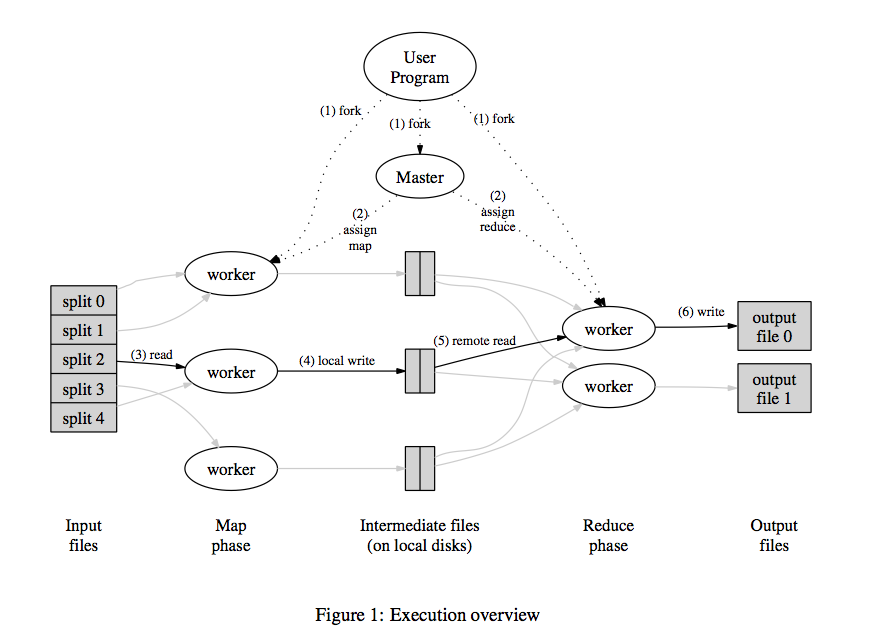
Workers read chunks, apply the maps. The worker gets the chunk information from the GFS master node and accesses the appropriate chunknodes. The results of maps are writted to intermediate files (usually locally, but wherever the master node says there is room). The reducers then start reducing, producing intermediate files along the way. At the end, output files are created, that can be distributed across many nodes! (remember, a file’s chunks can be anywhere in the GFS system). So, input data can be huge! (scalable to GFS limitations, which are super high), and output can even be huge!. Also, since the output is also files, the output can be used as input to further MapReduce jobs!

Of course, the system tries to keep data local and take advantage of rack infrastructure. Reducers are first run on a node, then nodes in the same rack are reduced (they share a router), then adjacent racks are reduced (to decrease router trafic), and so on.

Some examples (from the paper):

Bigtable

[GBT2008] So far, we have seen a general distributed file system approach to big data, coupled with a highly parallel mapreduce interface, but some key pieces are missing. First, a file system is very general, there is no notion of data types contained in files, only files, and the querying mechanisms are limited to standard file system operations. Second, mapreduce applies to a specific type of problem, and is not a good fit for every type of query. This is where Google’s Bigtable comes in. The basic idea of Bigtable is to provide a structured type mechanism for storing items, coupled with a general query mechanism. The general idea is that most of the application Google needed GFS for held data with some sort of structure. For example, a web page record will contain the link (its key), the contents of the page, and links of any web pages that link to that page. This is an extremely basic structure that requires some flexibility (web pages can have different lengths, some web pages will be linked to more than others), but can take advantage of typing, attribute names, and structure to make querying easier.

Bigtable is actually built on top of GFS.

Data Model

The data model is extremely simple... Big table is essentially a map (think data structure map, or hash table). The map is indexed by a (row key, column key, and timestamp) and returns a string. Row keys and column keys are strings, and the timestamp is an integer. Thus, all data is stored as strings, leaving a lot of flexibility. In fact, whatever data you want to store must be encoded into a string!:

Bigtable data map structure

Within a particular database, rows are maintained in lexicographic order by row key. Rows are broken into ranges, a single range is stored in a tablet (think file from GFS). Thus, the user can control to the locality of data by placing row keys near each other lexicographically. For example, a database of web pages can use URLS as row keys, and reverse their structure such that the TLD comes first, followed by the domain, followed by the subdomain. For example: com.cnn.money, com.cnn.health, etc.

Column keys are grouped into families, so that keys of the same family can be compressed and stored together. The intent is for the number of families to be small, but the number of actual colums to be potentially huge. At this point, you should disassociate the term column from any database connotation. In this sense, the family is analogous to a relational data base column, and the Bigtable column is actually a piece of data. Columns are specified by the following: family:data, where data is string.

Each cell (column) has a timestamp. Bigtable will keep a user specified number of outdated data versions, the garbage collector will collect any outdated copies that exceed that number.

So, the takeaway here is that Bigtable is meant to store collections such that a collection has a potentially huge number of rows. Each row will have a small number of families, but a potentially huge number of columns. Rows in a collection typically have the same families, but can have different numbers of columns, and each column can be of arbitrary length. So, some structure is implied, but it is up to the user to enforce the structure, not Bigtable. Also, if the user finds the structure must evolve over time, new rows in a collection can simply have different structure. The goal is a balance between structure and flexibility, an easy to use text-based data representation, and the ability to have huge rows, and huge numbers of rows.

Example: storing web pages.

In the paper, Webtable is used as an example. Webtable is a Bigtable database that stores web pages, and the URLs of sites that link to each web page. Each record has the following structure:

row key = [reversed url], contents:"<html> ... </html>", anchor:"url of a linking site" t2, ... , anchor:"url of a linking site" tn

A timestamp is stored with each column. Multiple versions of a single column can exist (with differing timestamps).

Assume cnn.com is linked to by cs.siue.com and active.com. The resulting record looks like:

Note that the number of anchors is variable depending on the website. Also, each anchor is variable length, and the web page contents are of variable length.

API

An API exists on top of Bigtable, and a mapreduce interface exists. Single row transactions are supported, which allows atomic read-modify-write sequences on a single row. General transactions are not supported.

General transactions were going to be a part of Bigtable, but none of the applications using Bigtable required them. The major source of requests for transactions is to support secondary indexes. Specific functionality to support secondary indexes is planned. This support will be more efficient than general transactions, but less general.

Implications

The ideas behind Bigtable have found their way into numerous products: MongoDB, Hive, Cassandra, etc. The notion of text based storage, a flexible structure, potentially huge rows (or documents, or whatever the various systems call them), is extremely powerful. Furthermore, because these systems are built on a GFS-type file system, all the advantages of GFS are there: data replication, commodity hardware, easy data replication across geography.

The main drawbacks are lack of enforceable structure of records (like relational databases provide), and lack of transactions (although later work addresses transactions).

If you look at the querying models provided by Bigtable like systems, you notice that they follow the mapping paradigm pretty closely. In general, such systems are referred to as key,value stores, since a key is mapped to a value (a row key maps to a row consisting of a bunch of columns). Other systems use the terminology that a key maps to a document. These systems have received much attention and use in a variety of web applications.

Note

What are some good examples of the use of key,value stores in applications?

Think about Facebook... They use a variety of systems to keep track of everything. Where does a key,value store fit in?

What are reasons to not use a Bigtable-like key,value store? Think beyond transactions. (Think about link pointers in B-trees)

Percolator [Perc2010]

Basic idea: MapReduce and batch processing systems are most efficient with big chunks of data, so a need exists to make small incremental updates. For example, web pages change somewhat frequently, how can those changes be reflected efficiently in GFS? Percolator addresses this issue, allowing the same number of documents to be processed per day as was before, but reducing the average age of documents in Google Search (by about 50%!).

The Problem

Building an index of the web.

1. Crawl every page on the web
2. Process them with respect to some invariants. Example: if a page is crawled under multiple URLS (multiple linking pages), only the one with the highest pagerank gets put in the index. (pagerank must be fixed during this step). Each link is inverted so that the anchor text from outgoing links is attached to the page to which the link points. This must also work across duplicates (links to a duplicate page are linked to the highest pageranked link)

This can be accomplished with mapreduce jobs. One to cluster duplicates, one for link inversion, etc. Note that this style of algorithm construction used natural barrier synchronization. One mapreduce job must finish before the next starts! This makes the invariants trivial to enforce!

What if we want to update the index after a crawl of a small portion of the web. The original way to do it: Re-run the entire process! Its doable, thanks to the scalability of GFS and mapreduce, but that wastes a lot of resources (time, power, etc). Latency for the update is proportional to the size of the repository, not the size of the update!

We need some sort of transactions. Data volume is too big for DBMSs. Bigtable is scalable, but does not allow the enforcement of the invariants listed above.

What is needed is a way to maintain invariants, but allow many, concurrent, small, incremental updates.

The scale of the repository is multiPB.

Term : snapshot isolation: All reads within a transaction see the same copy of the database

Term: ACID transactions: atomic, consistent, isolated, durable.

Percolator provides ACID snapshot isolation semantics.

Transactional overview

Percolator is built as a client application (remember, master, server client) on top of big table. Recall that bigTable uses tablet servers to retrieve tablets. Tablets are stored in GFS on chunkservers as files. Users can control the grouping of items in a bigTable table. BigTable provides per-row transactional support (by using timestamps). Percolator will provide multi-row tansactional support

Multiple versions of a data item are stored (bigTable’s version number). This provides snapshot isolation (reads occur at a given timestamp). Writes appear at a later timestamp.

Require locks. BigTable is used to implenmt locks. Locks are stored in columns for the row that they apply to. (remember, we can always add or remove columns since there is no strict schema).

Requires a timestamp oracle, to get monotonically increasing timestamps throughout the system.

Procedure:

• First phase is prewrite. try to lock ALL cells being written to. If another transaction is writing to a cell, ABORT! (snapshot isolation does NOT provide serializability, so we must abort). If any lock is not available, abort. (how does this compare to traditional databases?)
• Second phase . Get a commit timestamp from the oracle. release locks and make written data visible with a write-record value written to the cell.
• Reads that encounter a lock must wait for the lock to be released (data is being written to that cell). (because this is distributed, not all copies are updated at the same instant. A read may have started at a timestamp whose commit is still percolating through the system).
• Clients can fail (percolator clients), leaving bad locks around. Percolator will clean up locks once it is SURE that a client is dead. It cannot do this, so every transaction has a primary lock. A client cannot complete a transaction without owning the primary lock. If percolater thinks a client is dead, it just steals the primary lock.
• Note that all this means that performance will not be ideal, it turns out to be on the order of seconds, not acceptable in a DMBS, but perfectly acceptable here.

Performance

Implications

So now we have transactions! sort of. How do these transactions compare with traditional DBMS transactions?

How can constraints be implemented in this system?

[GFS2003]

(1, 2, 3, 4, 5) Sanjay Ghemawat, Howard Gobioff, and Shun-Tak Leung. 2003. The Google file system. In Proceedings of the nineteenth ACM symposium on Operating systems principles (SOSP ‘03). ACM, New York, NY, USA, 29-43. DOI=10.1145/945445.945450 http://doi.acm.org/10.1145/945445.945450

[GMR2004]

Jeffrey Dean and Sanjay Ghemawat. 2004. MapReduce: simplified data processing on large clusters. In Proceedings of the 6th conference on Symposium on Opearting Systems Design & Implementation - Volume 6 (OSDI‘04), Vol. 6. USENIX Association, Berkeley, CA, USA, 10-10.

[GBT2008]

Fay Chang, Jeffrey Dean, Sanjay Ghemawat, Wilson C. Hsieh, Deborah A. Wallach, Mike Burrows, Tushar Chandra, Andrew Fikes, and Robert E. Gruber. 2008. Bigtable: A Distributed Storage System for Structured Data. ACM Trans. Comput. Syst. 26, 2, Article 4 (June 2008), 26 pages. DOI=10.1145/1365815.1365816 http://doi.acm.org/10.1145/1365815.1365816

[Perc2010]

Daniel Peng, Frank Dabek, Large-scale Incremental Processing Using Distributed Transactions and Notifications, Proceedings of the 9th USENIX Symposium on Operating Systems Design and Implementation, USENIX (2010).