
Graphs
Graph Definitions
A graph  is tuple containing two sets: a set of vertices
 and a set of edges
 . Each edge is simply a tuple containing two vertices:
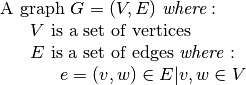
Because the edges are only defined as pairs of vertices, no concept of embedding space is implied by the definition of a graph. In fact, no concept of the location of a vertex is implied. For example, a vertex can be a point in 2D space, a number, a string, or anything else.
IF a graph is a directed graph, then direction of an edge is implied by the orering of the edge tuple (the source vertex is first, the destination is second). Otherwise, the graph is undirected and an edge implies a path in both directions between the vertices.
 and
 are adjacent if
 .
An edge may have a weight or a cost. The weight does not necessarily imply a distance between two vertices, but simply provides a value for an edge.
A path is a sequence of vertices  such that
 .
An edge  forms a loop.
A simple path contains distinc vertices, although the first and last vertices can be identical.
A cycle has at least 3 vertices and starts/ends on the same vertex. Edges in a cycle myst be distinct.
A graph is connected if there is a path to/from all pairs of nodes in the graph.
A directed graph that is connected is strongly connected. It is weakly connected if it is not strongly connected, but its underlying undirected graph is connected.
Examples
Airport systems: usually strongly connected.
- Vertices = airports
- Edges = direct flights
- Edges may have costs: distances, fuel costs, airport fees, likelihood of weather delays, etc.
Traffic flow:
- Edges = roads
- Vertices = intersections
- Costs: road congestion, road capacity, construction, etc.
Graph Representation
Adjacency Matrix:
Adjacency Matrix: A matrix  such that if edge
 then
 :

Excercise
Is the above graph strongly connected?
Is the graph weakly connected?
For weighted graphs, a non-connected edge is typically represented by a max or a min cost. The assumption is that the chosen cost will not show up in an actual graph.
Storage of an adjacency matrix is  . It is good for dense graphs in which the matrix is nearly or completely full. It is not so good for sparse graphs in which the matrix is mostly empty. A sparse matrix means we are allocating space to indicate the absence of an edge.
Real world graphs are often sparse:
Manhattan (not counting Broadway): intersections usually have 4 edges emanating.
4 edges pr intersection: 
if there are 3,000 intersections = 12,000 edges stored in 9,000,000 matrix cells. A lot of wasted space.
Adjacency List:
Adjacency List: For each vertex, keep a list of all adjacent vertices. Space complexity:  . For the example graph given above, the space would be
 instead of

The Adjacency list for the graph above is:
1: 2, 3, 4
2: 4, 5
3: 6
4: 6, 7, 3
5: 4, 7
6 :
7: 6
Concept
For a graph, linear space complexity means that the vertices and edges are stored a constant number of times, leading to . Similarly for linear computational complexity, the edges and vertices are visited a constant number of times.
Adjacency lists vs adjacency matrices?
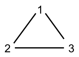
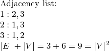
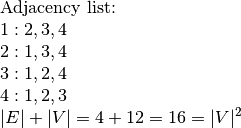
Adjacency lists are better for sparse graphs. For dense graphs, adjacency matrices tend to be better because the overhead of the node structure of linked lists is not present. Recall that a node must contain a pointer to the next node in the list, leading to more memory usage. For complete graphs (every edge is connected to every other edge), an adjacency matrix is preferable, in general.

Topology
In general, graphs can be considered to be embedded in topological space, as opposed to metric space. In metric space, there is a concept of distance (among other things). For example, we are used to dealing with the metric space  (i.e., Euclidean space), in which the concept of Euclidean Distance exists. For example, we can compute the distance between two points to determine how close or far they are apart,
Topological Space
In topological space, there is no concept of distance between points. So, points are either disjoint, or are equal; however, we cannot say if they are close or far because these concepts rely in distance measures. We can tread Euclidean space as a topological space if we choose.
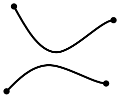
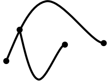
Topological Relationships are qualitative relationships among objects in a topological space. Assume the topological space . If two lines are embedded in that space, the following are some possible topological relationships.
Intersects:

Disjoint:
Meet:
Topology joke: A doughnut is topologically equivalent to a coffee cup: they are both solid objects that have a single handle. So... a topologist cannot tell the difference between his/her doughnut and coffee cup! This is why there are so few topologists around.
Although graphs are often considered to be embedded in a topological space, many useful graphs are actually embedded in geographic space. For example, road networks definitely have a concept of distance.
Exercise
Think about a road network, for example the blocks in Manhattan. Assume your location is known and you want to find the nearest gas station to your location. The algorithm will be very different if you consider the graph to be embedded in topological space or metric space. Sketch out the algorithm. Which one is faster? Which one returns more reliable results?
Topological Sort
Definition: A directed acyclic graph (DAG) is a directed graph that contains no cycles.
A topological sort of a DAG results in a list of vertices ordered such that if there is a path from  to
 in the graph, then appears before in the ordering. Note that due to this definition, there is no way to topologically sort a graph with a cycle.
A topological sort is not necessarily a total ordering or a unique order. In fact, it is much more like a lattice ordering. Vertices may exist such that one cannot say that one vertex must come before the other.
Example: Course sequences.
One can represent course sequences as a topological sort of a course prerequisite graph. For example, if cs111 and cs140 are prerequisites for cs314, but cs140 and cs111 have no prerequisites, then there are two possible topological sorts of the graph:
cs111, cs140, cs314
cs140, cs111, cs314
Both sorts are valid, and correct according to the graph. Specifically, cs140 and cs111 have no ordering implied by the graph that forces you to take one before the other; you can take them in any order. However, both cs111 and cs140 are less than cs314 in terms of the topological sort of the graph.
Definition: The in-degree of a vertex is the number of incoming edges to a vertex: 
The simple algorithm for computing a topological sort is as follows:
- Compute the in-degree of all vertices.
- Find a vertex with in-degree of 0. print it.
- Decrease the in-degree of all vertices with an incoming edge that comes from the just-printed vertex.
- repeat steps 2 and 3 until no more vertices with in-degree = 0 remain.
The simple algorithm has time complexity  since we must repeatedly scan all vertices to find a vertex with in-degree of 0. We can improve upon this by storing all vertices with an in-degree of 0 in a queue.
Topological Sort Algorithm (better)
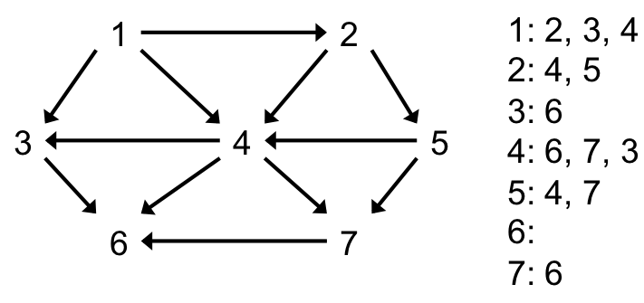
Algorithm:
- Compute the in-degree of all vertices.
- All vertices with in-degree=0 go into a queue.
- While the queue is not empty:
- ~Dequeue a vertex .
- ~Decrement edge counts for all neighbors of
- ~If the in-degree of a vertex falls to 0, enqueue it.
For the above the graph, the iterations of the algorithm look like the following:
| Vertex (v) | In-degree(v) | ||||||
| v1 | 0 | ||||||
| v2 | 1 | 0 | |||||
| v3 | 2 | 1 | 1 | 1 | 0 | ||
| v4 | 3 | 2 | 1 | 0 | |||
| v5 | 1 | 1 | 0 | ||||
| v6 | 3 | 3 | 3 | 3 | 2 | 1 | 0 |
| v7 | 2 | 2 | 2 | 1 | 0 | ||
| enqueue | v1 | v2 | v5 | v4 | v3,v7 | v6 | |
| queue | v1 | v2 | v5 | v4 | v3,v7 | v7 | v6 |
| dequeue (topological ordering) | v1 | v2 | v5 | v4 | v3 | v7 | v6 |
Time complexity:  . Scan all edges to create the initial in-degree list (scan the adjacency list). When a vertex is dequeued, use the adjacency list to find all vertices that must have their in-degree decremented (use a hash table, array index, or other constant time lookup structure to store the in-degree values). Each vertex is enqueued and dequeued exactly once.
Remember, topological sort is a is a graph induced ordering. Metric ordering is an embedded-space-induced ordering on the vertices, but does not necessarily reflect the graph.
Note: What does it mean if you get to a point where no vertex has an in-degree of 0?
Unweighted Shortest Path
Definition: The unweighted shortest path problem is stated as: given a source vertex in a graph, find the shortest paths to all vertices.
Strategy: Use a Breadth First Search (BFS) approach. The basic idea is to find all vertices that 1 edge away from the source, then 2 edges away, then 3 edges away, etc. This is in contrast to depth first search in which we would travel as far as possible along a path until it completes before we begin a new path. For example, a BFS of a binary tree would visit the root, then all nodes at level 1, then all nodes at level2, etc. The depth first search would travel all the way from the root to a leaf, then to another leaf, then to another leaf, etc.
Algorithm: Find the neighbors of a source vertex, add 1 to their path length. Get the neighbors of those, and add one to their path length, etc.
Improvement: Just like the topological sort, uses a queue and adjacency list to achieve linear time complexity. Simply enqueue the source vertex. Each iteration, dequeue a vertex, add 1 to its path length, and add its neighbors the queue. Effectively, all vertices 1 hop away from the source will show up first in the queue, followed by all vertices 2 hops away from the source, followed by all vertices three hops away, etc.
Unweighted Shortest Path Example:
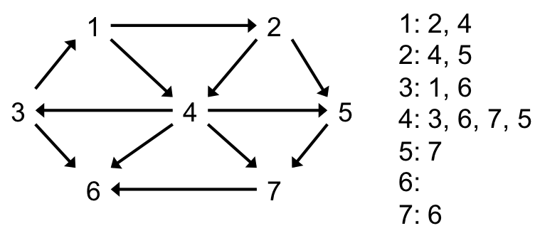
Example, find all shortest paths from v3:
K = known
PV = previous vertex
DV = distance value
| Vertex | K | PV | DV | K | PV | DV | K | PV | DV |
|---|---|---|---|---|---|---|---|---|---|
| v1 | T | v3 | 1 | ||||||
| v2 | F | x | T | v1 | 2 | ||||
| v3 | T | v3 | 0 | ||||||
| v4 | F | x | T | v1 | 2 | ||||
| v5 | F | x | F | T | v4 | 2 | |||
| v6 | T | v3 | 1 | ||||||
| v7 | F | x | F | T | v4 | 2 | |||
| enqueue | 6,1 | 4,2 | 3,6,7,5 | ||||||
| queue | 6,1 | 4,2 | 2,3,6,7,5 | ||||||
| dequeue | 6,1 | 4 | 2 | ||||||
Note that 3,6,7,5 area all known when they are dequeued in the final iterations.
Dijkstra’s Algorithm
See Notes and Book
Prim’s Algorithm (MST)
See Notes and Book
Kruskal’s Algorithm (MST)
See Notes and Book
Euler Circuits
See Notes and Book