Sum3 Problem Overview

Basic Description

The Sum3 problem is described by a rather simple question: Given a set of integers, how many triples of distinct elements in that list add up to 0.

For example, given the following list:

-1, -2, 0, 2, 3

the answer is 2:

-1 + -2 + 3 = 0
-2 + 0 + 2 = 0

The simplest way to code a solution to the Sum3 problem is to use a double nested looping structure to generate the indices of all possible triples in the input array. Clearly, this is simple to express in code, but has an unfortunate time complexity of . For example, the following C++ code uses 3 for loops to achieve a correct solution.

#include <iostream>
using namespace std;

int main( )
{
        int dataSize = 5;
        int* data = new int[ dataSize ];
        data[0] = -1;
        data[1] = -2;
        data[2] = 0;
        data[3] = 2;
        data[4] = 3;
        // do the naive Sum3 computation.  O(n^3)
        int count = 0;
        for (int i = 0; i < dataSize-2; i++)
                for (int j = i+1; j < dataSize-1; j++)
                        for (int k = j+1; k < dataSize; k++)
                                if (data[i] + data[j] + data[k] == 0)
                                        count++;

        cout<< count <<endl;

}

Complete Naive Solution

The next code block uses the same solution as above, but includes a command line parameter that will generate an array of random numbers of a user-specified size. The getRandInt() function loads the vector passed into it with random integers. The data vector allocates space for the number of integers required, and is then passed to the getRandInt() function. This version of the program allows the user to get a feel for how and program behaves in practice. Try compiling the program and running it.

#include <iostream>
#include <sstream>

using namespace std;

int getRandInt( int* dataVec, int dataSize )
{
        // load up a vector with random integers
        int num;
        for( int i = 0; i < dataSize; i++ ) {
                // integers will be 1-100
                num = rand() % 100 +1;
                if( rand( ) % 2 == 0 ) {
                        // make some integers negative
                        num *= -1;
                }
                dataVec[i] = num;
        }
}


int main(int argc, char * argv[] )
{
        int dataSize = 0;

        if( argc < 2 ) {
                std::cerr << "usage: exe  [num of nums] [optional seed value]" << std::endl;
                exit( -1 );
        }
        {
                std::stringstream ss1;
                ss1 << argv[1];
                ss1 >> dataSize;
        }
        if( argc >= 3 ) {
                std::stringstream ss1;
                int seed;
                ss1 << argv[2];
                ss1 >> seed;
                srand( seed );
        }
        else {
                srand( 0 );
        }

        // create a data vector
        int* data = new int[ dataSize ];

        // load it up with random data
        getRandInt( data, dataSize );
        int *dataPtr = &data[0];
        // do the naive Sum3 computation.  O(n^3)
        int count = 0;
        for (int i = 0; i < dataSize-2; i++)
                for (int j = i+1; j < dataSize-1; j++)
                        for (int k = j+1; k < dataSize; k++)
                                if (dataPtr[i] + dataPtr[j] + dataPtr[k] == 0){
                                        count++;
                                }
        cout<< count <<endl;
}

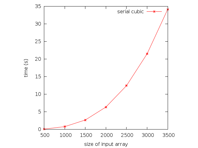
Here are some running times for the previous program:

Array Size	Time (s)
500	.106
1000	.804
1500	2.698
2000	6.382
2500	12.459
3000	21.519
3500	34.162

The running times are plotted. The cubic nature of the curve is clearly visible.

Exercise

Create a Makefile and use the Makefile to compile the program listed above. Run the program using the time command on linux to see some running times. Collect running times on two different machines. Write a brief report indicating your results and listing the machine specifications. List reasons why one machine is faster than the other.

To find out machine specs on linux, check out the lspci abd lscpu commands, and check out the /proc filesystem. Check the man pages and/or google for information on how to use/interpret these resources