Trees

Unbalanced Binary Trees

Binary Trees

Definition

For a binary tree:

A tree is a:

• empty tree.
• an item.
• an item followed by trees.

For an n-ary tree:

A tree is a:

• empty tree.
• an item.
• an item followed by trees.

Note the recursive nature of the definitions. Recursion is a natural fit for trees.

A forest is a group of 2 or more trees

A binary tree API typically has the following operations:

• create a tree
• isEmpty
• contains( value )
• traverse // often through iterators
• remove item
• add item

Tree Traversals:

There are 3 classic tree traversals: pre-order, in-order, and post-order. They are summarized in the following code snippets:

preorder(node) {
        visit(node);
        preorder(node.leftChild);
        preorder(node.rightChild);
}

inorder(node)
{
        inorder(node.leftChild);
        visit(node);
        inorder(node.rightChild);
}

If items in the tree are sorted (in a binary search tree), in-order visits items in order

postorder(node)
{
        postorder(node.leftChild);
        postorder(node.rightChild);
        visit(node);
}

Post-order is useful for printing a tree such that the structure is visible.

For the following tree:

pre-order:HDBACFEGPKINURY

in-order: ABCDEFGHIJNPRUY

post-order: ????

Note about recursion

Recursion if often frowned upon in production code. Why?

What are the advantages of recursion?

What are the disadvantages of recursion?

If you need a recursive function, but you don’t want some of the disadvantages of recursion (call stack limitations), you can essentially implement the stack yourself. In other words, use an iterative function, but push and pop data onto a stack to simulate recursion. This allows much more efficient stack management (less overhead) and larger stack sizes.

A last note. Binary trees can be implemented as arrays rather than node structures.. For example:

To compute the children of node with array index :

Array construction of binary trees is super useful for complete or nearly complete trees. One issue to consider is how to tell if a node is empty (essentially, detect a null pointer)?

Array construction of binary trees will be super useful later.

Binary Search Trees

Definition

A binary search tree is a binary tree where each node contains an item such that a total ordering exists over the items. Furthermore, for any node containing item , all items in the left subtree from are less than or equal to , and all items in the right subtree from are greater than

Thus, the binary search tree must preserve both tree structure, and the order of the items.

Typically, binary search trees are used for searching for items

Search operation: Look at a node to see if it has the value we want, if what we are looking for is less than the value, visit the left subtree, otherwise visit the right subtree.

Insert operation. Perform a search, but continue until we hit a leaf. Insert the item at the leaf. inserting at leaves is EASY, inserting in the middle of the tree is hard. we see this a lot with trees

Exercise

Insert the following into a binary search tree. Show the tree at each step:

9, 6, 8, 7, 3, 0, 10, 5

Remove operation: The easiest method is the remove from a leaf (just like with insert). So the general idea is copy whatever we want to delete to a leaf, then delete the leaf. Sometimes, we cannot find a leaf, so we must simply find a node with a single child pointer (which is an easy case to handle)

One problem, we must exchange the value of a node with a value in a leaf. And, we must do this while preserving the tree ordering (after the delete of course). So, we need to identify either the previous or successive value in the tree with respect to item ordering. Luckily, there is an easy formula to find these.

Finding the next/previous value in sequence in a BST for the delete operation

Consider the following tree:

The value in the tree immediately less than 9 can be found by visiting the left child of the node containing 9, then following right child pointers until a NULL pointer is found

The value in the tree immediately greater than 9 can be found by visiting the right child of the node containing 9, then following left child pointers until a NULL pointer is found.

Note that in this case, if we want to delete 9, we can swap it with 8, resulting in:

To delete the node that now contains 9, we can simply connect the right child of the 6 node to the 7 node (because the 9 node only has 1 child):

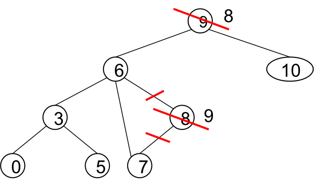
The idea is simply to never delete a node with 2 children.

Note that the structure and order is maintained in the tree.

Finally, the time complexities of BST operations are related to the height of the tree. Why?

What are the worst case and best case time complexities of search, insert, and remove?

Balance and BSTs

BSTs are NOT guaranteed to be balanced, but, if the input is inserted in a random order, they tend to be. For BSTs, randomness is your friend. Although there is no guarantee of balance, if the input is expected to be random, you can expect logarithmic operation time.

However, deleting from a BST tends to degrade randomness an favor more unbalanced trees. BSTs can be a very good and simple choice. There tends to be costs to achieve balance.

Balanced Trees

For operations on trees, the worst case cost of the operation is equivalent to the height of the tree. For a BST with items inserted in random order, the costs is roughly . Items inserted roughly in order lead to costs of . Insertions and deletions tend to make things worse (less random).

Instead of relying on the randomness of data ordering, lets look at some trees that are guaranteed to be balanced. The guarantee balance comes with a price, these trees are significantly more difficult to implement than traditional BSTs.

Definition: Balanced Tree

A balanced tree is a tree that is close to its minimal possible height (its longest branch is close to the minimal possible height for the number of items in the tree). For items, a balanced binary tree will have height close to , a trinary tree will have height close to , an k-ary tree will have height close to .

2-3 Trees

A 2-3 tree node has space to hold 2 items and 3 pointers. A node will always have 1 item and 2 pointers (a 2 node), or 2 items and 3 pointers (a 3 node):

Items in nodes are ordered. So, the first item is always less than or equal to the second item (if there are 2 items in the node). Searching for a value is similar to a BST, except there are 3 possible pointers to follow. The algorithm is as follows

find( node*, item):
 is the item in the first slot?
 if Yes: done
 if No: Is the item less than item in first slot?
    if Yes: find( node.leftChild )
    if No: Is the item in second slot?
       if Yes: done
       if No: is the item less than item in second slot?
          if Yes: find( middleChild, item )
          if No: find( rightChild, item )

Inserting into a 2-3 tree

The 2-3 tree is guaranteed to ALWAYS be balanced. Therefore, we cannot simply insert items by creating new leaves like we do with a BST. The process is as follows:

• Always insert a new item at a leaf, but never increase the depth of the tree at the leaves.
• Use the search algorithm to find the leaf that a new item should go in.
• If it is a 2 node, then just put the item there.
• If is a 3 node, split the node into 2 nodes, and promote the middle of the 3 values up to the parent node.
• If the parent does not have room (it is already a 3 node), split that node and promote the middle value to its parent. Recursivley repeat until no splittting occurs.

If this procedure is followed, the height of the tree will be increased at the TOP of the tree (the root). Basically, tree height will increase once a root is split. An example follows:

Example 2-3 Tree Insertion

Insert the following: 10 40 20 5 15 17 19

On paper, the insertion algorithm is not too bad. By drawing pictures, you can usually figure out where things should go. Actually implementing the code is anoother story. The following is a working 2-3 tree implemenation. Try to summarize the portions of the code in pseudo-code. Make sure you know what each code block is doing. The downloadable source file is here

class node:
    def __init__( self ):
        self.data = [None, None]
        self.next = [None, None, None]
        self.size = 0

    def __str__(self ):
        return   str( self.data ) + '(node has '+ str( self.size ) + ' item(s))'

class tree23:
    def __init__( self ):
        self.head = None
       
    def insert( self, item ) :
        #special case: empty
        if self.head == None:
            self.head = node()
            self.head.data[0] = item
            self.head.size = 1
            return

        # find leaf
        # leaf will ALWAYS have next[0] == None
        ptr = self.head
        myStack = [ ptr ]  #keep a stack of nodes visited back up to the root
        while( ptr.next[0] != None ):
            if item < ptr.data[0]:
                nextIndex = 0
            elif ptr.size == 2 and item > ptr.data[1]:
                nextIndex = 2
            else:
                nextIndex = 1
            ptr = ptr.next[ nextIndex ]    
            myStack = myStack + [ptr]

        #pop the current node off the stack
        myStack.pop()
        
        print 'INSERT -- we have found a leaf:', ptr
        # now we are at a leaf.  If we have room, just put it in
        if ptr.size == 1:
            insertIndex = 0
            if item > ptr.data[0]:
                insertIndex = 1
            #shift data, and put the new value in
            ptr.data = ptr.data[(-1*(insertIndex+1)):] + ptr.data[:(-1*(insertIndex+1))]
            ptr.data[insertIndex] = item
            ptr.size +=1
            return

        print 'INSERT -- leaf is full, must split a node'
        # final case, node is full.  
        # make a new sibling and parent.  Set up the nodes
        # we are at a leaf, so we don't need to worry about pointers
        leftNode = node()
        leftNode.size = 1
        rightNode = node()
        rightNode.size = 1
        parNode = node()
        parNode.size = 1
        # assign data and pointers
        if item < ptr.data[0]:
            leftNode.data[0] = item
            parNode.data[0] = ptr.data[0]
            rightNode.data[0] = ptr.data[1]
        elif item < ptr.data[1]:
            leftNode.data[0] = ptr.data[0]
            parNode.data[0] = item
            rightNode.data[0] = ptr.data[1]
        else:
            leftNode.data[0] = ptr.data[0]
            parNode.data[0] = ptr.data[1] 
            rightNode.data[0] = item
            
        parNode.next[0] = leftNode
        parNode.next[1] = rightNode
        if len(myStack) == 0 :
            # we are splitting the root
            self.head = parNode
            return

        # At this point, we have made a new sub-tree by splitting a node.  
        # parNode is the parent of the sub-tree

        # now merge the parnode with the parent.  possibly recursively splitting
        done = False
        while len( myStack) > 0 and not done:
            theParent = myStack.pop()
            print'INSERT -- splitting back uip the tree at parent node:',  theParent
            # if we have room in the parent node, merge it with parNode
            if( theParent.size == 1 ):
                 insertIndex = 0
                 if parNode.data[0] > theParent.data[0]:
                     insertIndex = 1
                 #shift data, and put the new value in
                 theParent.data = theParent.data[(-1*(insertIndex+1)):] + theParent.data[:(-1*(insertIndex+1))]
                 theParent.next[2] = theParent.next[1]
                 theParent.data[insertIndex] = parNode.data[0]
                 theParent.size +=1
                 theParent.next[insertIndex] = parNode.next[0]
                 theParent.next[insertIndex+1] = parNode.next[1]
                 done = True
                 break
            else:
                # need to merge the nodes
                # Each time through here we already have the sub tree built
                # we are just merging its root node with the parent node that was
                # pointing at the subtee we are working on.
                # parnode is the node to be merged.  Its children are already set
                # theParent is the node parNode must be merged with
                # promote node is the node of the data that will be promoted up since
                # we only get here if theParent is full
                promoteNode = node()
                if parNode.data[0] < theParent.data[0] :
                    print 'small'
                    promoteNode.data[0] = theParent.data[0]
                    promoteNode.next[0] = parNode
                    promoteNode.next[1] = theParent
                    promoteNode.size = 1
                    theParent.data[0] = theParent.data[1]
                    theParent.size = 1
                    theParent.next[0] = theParent.next[1]
                    theParent.next[1] = theParent.next[2]
                    parNode = promoteNode
                    continue
                elif parNode.data[0] < theParent.data[1] :
                    print 'med'
                    promoteNode.data[0] = parNode.data[0]
                    promoteNode.next[0] = theParent
                    promoteNode.next[1] = parNode
                    promoteNode.size = 1

                    theParent.size = 1
                    theParent.next[1] = parNode.next[0]
                    
                    parNode.data[0] =theParent.data[1]
                    parNode.next[0] = parNode.next[1]
                    parNode.next[1] = theParent.next[2]
                    parNode.size = 1

                    parNode = promoteNode
                    continue
                else:
                    print 'big'
                    promoteNode.data[0] = theParent.data[1]
                    promoteNode.next[0] = theParent
                    promoteNode.next[1] = parNode
                    promoteNode.size = 1
                    theParent.size = 1
                    parNode = promoteNode
                    continue
        # if we never set done, then we broke all the way up to the root node
        # so reset the root pointer
        if not done:
            self.head = parNode

    def printTree( self ):
        self.printRecursive( self.head, 0 )
	
        
        
    def printRecursive( self, curr, depth ):
        # post order traversal
        # print right child, middle child,  left child, then the current node

        # base case for recursion
        if curr == None:
            return

        # the following string will allow us to indent the nodes properly
        aString = ['\t']*depth # make a list of a bunch of tab characters
        aString = ''.join( aString ) #convert the list into a string for printing
        
        printedNodeDelimiter =False
        if curr.size == 2:    # if it isa 2 node, handle the rightmnost pointer and right most data
            self.printRecursive( curr.next[2], depth+1 ) #recursively print the tree
            print aString, '~'   # a character to mark the node
            printedNodeDelimiter = True
            print aString, curr.data[1]
        self.printRecursive( curr.next[1], depth+1 ) #recursively print the tree for the middle pointer
        if not printedNodeDelimiter:
            print aString, '~'   # a character to mark the node
        print aString, curr.data[0] # print the left most data
        print aString, '^'   # a character to mark the node
        self.printRecursive( curr.next[0], depth+1 ) #recursively print the tree for the left pointer


                
t = tree23()

t.insert( 1 )
t.printTree()
print '---------------------'
t.insert( 2 )
t.printTree()
print '---------------------'
t.insert( 3 )
t.printTree()
print '---------------------'
t.insert( 4 )
t.printTree()
print '---------------------'
t.insert( 5 )
t.printTree()
print '---------------------'
t.insert( 6 )
t.printTree()
print '---------------------'
t.insert( 7 )
t.printTree()
print '---------------------'
t.insert( 3.5 )
t.printTree()
print '---------------------'
t.insert( 3.7 )
t.printTree()
print '---------------------'
t.insert( 9 )
t.printTree()
print '---------------------'
t.insert( 1.2 )
t.printTree()
print '---------------------'
t.insert( 1.4 )
t.printTree()
print '---------------------'
t.insert( 3.1 )
t.printTree()
print '---------------------'
t.insert( 3.2 )
t.printTree()
print '---------------------'
t.insert( 3.3 )
t.printTree()
print '---------------------'
t.insert( 3.4 )
t.printTree()
print '---------------------'

Delete: Deleteing from a 2-3 tree is super tricky. Consider the following example. We can’t delete in that fashion because it breaks the search algorithm!

The basic idea to delete from a 2-3 tree is to do something similar to BST delete, but to enforce balancing. Basically, move the item to be deleted to a leaf node. Thenremove the item. Then, if a node is empty, recursively merge nodes up the tree (possible shortening the tree). Merging nodes is a pain, and there a lot of special cases to code. Typically, you try to avoid merging by stealing data from other nodes, but this sut leads to more special cases to code. We will not focus on 23 tree delete.

Roundup:

• Pro: 2-3 trees are balanced! insert, search, delete are all .
• Con: Super hard to implement, especially delete.
• Con: Nodes are not all full (wasted space?), but we get a balanced tree.
• Con: Hard to debug.

So, 2-3 trees are a nice introduction to balanced trees because they succinctly summarize the tradeoffs faced by all balanced trees: balanced trees are HARD to implement (especially fully with delete, etc). But, we get good guaranteed worst case performance!

2-3-4 Trees

One reason that 2-3 trees are so difficult is that is that when splitting/combining nodes, we end up having 3 items to deal with, but only space for 2 in a single node. This just makes things more difficult. 2-3-4 trees are similar to 2-3 trees, but allow 1, 2, or 3 items per node, alleviating that particular problem. Furthermore, we will implement the splitting strategy with a different philosophy to avoid recursive node splitting, greatly simplifying the code.

2-3-4 Tree Definition:

A 2-3-4 tree is a height balanced search tree such that the leaves of the tree are all at the same depth. A node can contain 1, 2, or 3 items and 2, 3, or 4 pointers. Items in a node are sorted, and an item is always surrounded by valid pointers (except for leaf nodes).

The node is structured as follows:

class node:
        def __init__(self):
                self.data = [None, None, None]
                self.ptr = [None, None, None, None]

The height of the tree will be somewhere between and :

• Balanced binary trees height
• Balanced tri-nary trees height
• Balanced quad-nary trees height

Insert Algorithm:

Like a 2-3 tree, always insert at a leaf.

Recall that inserting into a 2-3 tree is complicated mainly because of the recursive code. We will take a different philosophy for 2-3-4 trees. Instead of recursively splitting, we will preemptively split full nodes as we descend the tree, so we will NEVER have to recursively split a node.

Thus, the algorithm is as follows:

Get the root node
If the root is full:
        split the root, assign items and pointers
Get the pointer P to the appropriate child node.
while P is not null:
        if P is full:
                 split the node pointed to by P, assign items and pointers
        if P is a leaf:
                 add the item to the appropriate spot in P (it will always have room)
                 P is assigned NULL (break out of the loop)
        else:
                 Get the pointer P to the appropriate child node

Lets see an example:

Exercise: Implement 2-3-4 Tree Insert

Here is a skeleton to get you started. I have essentially implemented the easy parts of the pseudocode above, and left the hard parts to you. One thing to note is that because we preemptively split down the tree, there are only 2 cases that need to be handled for insert.

class node:
        def __init__(self):
                self.data = [None, None, None]
                self.ptr = [None, None, None, None]

        def isLeaf(self):
                return self.ptr[0] == None

        def getDataIndex( self, data ):
                if self.data[0] == None:
                        return 0
                elif data <= self.data[0]:
                        return 0
                elif self.data[1] == None:
                        return 1
                elif data <= self.data[1]:
                        return 1
                else:
                        return 2
        def getPtrIndex( self, data ):
                if data <= self.data[0]:
                        return 0
                elif self.data[1] == None:
                        return 1
                elif data <= self.data[1]:
                        return 1
                elif self.data[2] == None:
                        return 2
                elif data <= self.data[2]:
                        return 2
                else:
                        return 3

class t234:
        def __init__( self ):
                self.root = node()

        def splitRoot(self, nodePtr):
                if nodePtr.data[2] == None:
                        return nodePtr

                # Your code here

                return newRoot

        def split( self, nodePtr, index ):
                if nodePtr.ptr[index].data[2] == None:
                        return

                # Your code here


        def insert( self, data ):
                #check the split for root
                self.root = self.splitRoot( self.root )
                curr = self.root
                while curr != None:
                        #check if we are at a leaf
                        if curr.isLeaf():
                                index = curr.getDataIndex( data )
                                #for i in range(  len( curr.data)-1, index, -1 ):
                                #       curr.data[i] = curr.data[i-1]
                                curr.data[(index+1):] = curr.data[index:2]
                                curr.data[index] = data
                                return
                        else:
                                #find pointer to follow
                                index = curr.getPtrIndex( data )
                                self.split( curr, index )
                                index = curr.getPtrIndex( data )
                                curr = curr.ptr[index]

        def printTree( self ):
                self.printRecursive( self.root, 0 )

        def printRecursive( self, curr, depth ):
                #print right to left, then curr
                if curr == None:
                        return

                # Finish the print function


testWords = ['banana', 'apple', 'carrot', 'lettuce', 'pepper', 'kljdfg', 'sdflkj', 'fdgijerl', 'reoijht', 'troiu', 'ertoij', 'erwt', 'erty', 'ezz', 'exa', 'oerijfgdkm', 'sdff', 'qwer']

print testWords
print sorted( testWords )

DELETE

Deleting from a 234 tree is, again, hard. The idea, again, is to move the item to delete to a leaf, then remove it from the leaf. So, you swap the item to delete with its in-order successor. Then delete the item. If the node is then empty, you must merge nodes, again maintaining the tree properties of being perfectly balanced. Because you have 3 items in a node, it is possible to steal items from a neighbor.

Roundup:

The 234 tree is easier to implement than a 2-3 tree, but still tough, especially with delete. Again, there are lots of special cases with the delete algorithm that must be handled.

• Pro: height balanced, so good performance
• Con: increased memory usage (possibly 2 empty items and 3 empty pointers in every node)
• Con: still hard to debug

B+ trees

Disk Architecture Review

The hard disk is considered part of the memory hierarchy in computers (it is used to implement virtual memory). A typical memory hierarchy is:

Hard disks are typically the rotating magnetic platter type (SSDs are too expensive to completely replace them). Thus, HDs are the only mechanical device in your computer (other than fans and the DVD drive), and thus are the SLOWEST! HD access times are so long that computer users notice it takes a long time (think booting up the computer).

Because HD access times are so long, any data structure that needs to work well in a disk environment must be designed specifically for disk interaction.

Purpose:

• Long term, nonvolatile storage
• Lowest level in the memory hierarchy
• slow, large, inexpensive

General structure

• A rotating platter coated with a magnetic surface
• A moveable read/write head to access the information on the disk

Typical numbers:

• 1 to 4 platters (each with 2 recordable surfaces) per disk of 1” to 3.5” in diameter
• Rotational speeds of 5,400 to 15,000 RPM
• 10,000 to 50,000 tracks per surface
• cylinder - all the tracks under the head at a given point on all surfaces
• 100 to 500 sectors per track. The smallest unit that can be read/written.

B+ trees:

B trees and (more commonly used) B+ trees are a generalization of 2-3-4 trees to nodes with larger amounts of items and pointers. They are typically used for external memory search trees (in DATABASES!). Thus, they are typically referred to as an index structure. An index structure is simply database terminology for a data structure that provides faster data access than simply iterating through all items in a collection. B+ trees provide:

1. An index structure that is seperate from the data.
2. Hard lower and upper bounds on size and time to complete operations
3. Design specific to disk based structures.

B trees and their variants are used in virtually every DBMS out there.

We need a concept of a key that uniquely defines a record (basically an item). We will store complete records in one file (the relation). We will create a new file to hold the index. The index will contain keys that identify records, and the disk address of that record in the relation’s file. This means we don’t need to re-order the relation’s data file ever, we can simply append to it. Also, we can create as many index files as we want for whatever we want to search on.

We will talk about B+ trees, they are easier to use and manage, and work more naturally.

B+Tree

A B+tree contains 2 types of nodes: internal nodes and leaf nodes.

• internal nodes contain keys and pointers to other internal nodes or leaf nodes.
• leaf nodes contain keys and disk addresses of records in the relation’s data file.

A node is fixed size. Usually, a node is the size of a disk page. Sometimes it will be a multiple of the size of a disk page. This means the number of items stored in a node is dependent on the size of the item, and the size of the disk page (usually 4k).

let be the branching factor of nodes in a B+tree. indicates the number of child nodes for a node in the tree. Let be the actual number of keys in a node. For internal nodes . For leaf nodes: . Exceptions are made for the root node if there are simply aren’t enough items in the tree to reach the minimum threshhold.

Node Structure: Each node contains the following structure: [pointer, key, pointer, key, pointer, ..., key]. Pointers in internal nodes point to other nodes. Pointers in leaf nodes contain disk addresses, expect for the last pointer which points to the next successive node to the “right” in the tree

Note in B+ trees, keys are repeated in internal nodes and in leaves. This means every key will show up in a leaf. Some keys will show up in internal nodes. This is a major difference with standard B Trees

Searching the tree. Search the tree like a binary search tree

Insertion Into the Tree

1. Find the node at which to insert the item
2. If there is room in the node, insert it.
3. If there is no room, find the median value .
4. Create two new nodes, place all keys in the left node, and all keys in the right node.
5. Move the median value up to the parent node of the split node, and connect the tree. If there is no room for the median value in the parent node, repeat steps 4-5 on that node

B and B+trees are complete trees. They do not grow at the leaves, instead, they grow from the root!

Example

Put the following keys into a B Tree and a B+Tree. Let the branching factor :

20 5 8 40 23 31 1 10 33 41 22 7 16 44 27 35 11 9 2 17

How many nodes are visited to find the value 20? 33? 44?

How many nodes are visted to traverse the tree starting with value 31?

what is the time complexity of search and insert?

The algorithm for searching and inserting into a B+tree is straightforward, but the implementation of insertion can be tricky. In the worst case, a split can propogate up the entire tree to the root. It is useful to keep track of a stack of node pointers that lead back from the node of insertion ot the root.

As with most trees, the time complexities of the tree are dependent upon th tree height, for B+trees, the tree is always balanced, but trees with more full nodes might be shorter than trees holding the same amount of data with less full nodes.

For example, a B+tree with branching factor and height can have :

• at most pointers to data records. why?
• at min pointers to data records. why?
• a height bound for elements of , meaning logarithmic search, insert and delete!

Example

Assume a 4096 (4Kb) disk page and records with integer keys (4 bytes). Assume a 64 bit system (8 byte memory pointers). If B+tree blocks contain no header information, the we have keys per block (1 pointer and 1 key takes 12 bytes. the -8 is for the last pointer).

Lets assume a typical block will have 255 keys (somewhere between 340 and 340/2=170).

• With a root, we can store 255 pointers to records
• With a root and 255 leaves, we have pointers to records
• with a root and 255 internal nodes and 255 leaves for each internal node, we have pointers to records

So, such a B+tree with height 3 requires 3 disk accesses to search 16.6 mil records! Furthermore, the top few levels of a B+tre are typically buffered in memory, eliminating the need to disk access in may cases.

B+ Tree Delete

Again, like the 23 and 234 trees, delete is hard. In fact, because B+trees are used in databases, delete is often not worth it to implement. Instead, we use a lazy delete scheme. Instead of deleting and re-balancing, just mark an item as being deleted, and hopefully reuse the space later. Databases are in the business of remembering information, so delete should not happen too often. Think of an example.

A problem with this is wasted space, but hard drives are CHEAP!, so it is not such a problem.

I/O Complexity

We now have a new type of complexity, I/O complexity. Because disk access takes so long, the point is to have few I/O operations, and not worry too much about the in-memory stuff.

So, for a B+ tree with min nodes and max nodes and block size (disk page size) of :

• Number of leaf blocks is
• IO complexity for all operations is
• Height of tree is
• Time complexity to find is between
• Where is the time to find an element in a node

A final note when dealing with data that is big: Always remember your bandwidth

http://hothardware.com/News/Homing-Pigeon-Faster-Than-Internet-in-Data-Transfer/

Time to transfer  4GB   at 2.04MB per second  is ……
                4 hours, 39 minutes, and 37 sec

Time to transfer 2.57 PB == 2570000GB at 2.04Mbits per second is
                130821 Days 12 Hours 32 Minutes 13.54 Seconds == 358 years!

Size of a hard drive: .01 cubic foot

Cargo capacity of a Toyota Yaris: 25.7 cubic feet

Number of hard drives I can transport: 2570

If these are 1 TB hard drives, that’s 2.57 PB == roughly 20.56 peta bits

Time to drive to Chicago: 5hrs == 18000 seconds

Which gives a bandwidth of  1.14 Tbits/second   == 142  GB/second

And so the saying is: “Never underestimate the bandwidth of a station wagon
loaded with hard drives hurtling down the highway at 70mph”

Red Black Trees (RBTs)

2-3-4 trees are nice, but have some significant drawbacks:

1. they are hard to implement fully.
2. they have potentially a lot of wasted space in the nodes
3. delete is still a nightmare

A nice idea is to have the 2-3-4 tree advantages in a binary tree format. This is the idea behind red-black trees. Basically, for every 234 tree, there is an equivalent RBT. Basically, we are going to split up the 3 and 4 nodes into a group of binary nodes. The connected binary nodes are said to be connected with RED links, and the other links are black links. For example, a mapping between 234 and RB nodes follows:

Note: because red links are ,in some sense, internal node links in the 2-3-4 tree, there can never be 2 consecutive red links on a root to leaf path through the tree!

Note: black links are pointers in the 2-3-4 tree, so if we compress the red links to re-create the 2-3-4 tree, all the tree height properties still remain:

Properties

number of nodes

tree height

height of tree with red links compressed (height of the equivalent 2-3-4 tree)

• Property:
• Property:
• Property:

So, tree height is

With this style of implementation, the drawbacks to 2-3-4 trees (mostly) disappear. At least the wasted space disappears. Implementation is non-trivial, but easier than 2-3-4 trees.

So, a RBT node must contain an extra bit of information that records the color of the incoming link to each node.

Insertion Algorithm

Perform an insertion identical to binary search tree insertion (insert at the leaf! just like a 2-3-4 tree)
Color the incoming link to the newly inserted node RED
If the parent node of the newly inserted node also has a RED link coming into it, then we have 2 consecutive red edges
        Fix the problem using rotations and promotion!

Fixing the Tree!

If the tree is unbalanced after an insertion, we perform rotations and promotions to fix it. Here are the cases:

Key:

• G is the grandparent of the inserted node
• P is the parent of the inserted node
• N is the newly inserted node

Case 1: No violation

Case 2: The incoming edge of P is red and its sibling is black

Case 2.5: Same as Case 2, but the value of N falls in between the value of P and the value of G in sequence

Case 3: The incoming edge of P is red and its sibling is also red. This is called a promotion. This will only occur after a rotation has already taken place. It may have to be recursively repeated up the tree.

Summary:

If 2 consecutive red edges are present immediately after an insertion, perform a rotation to restructure the tree. Only ONE rotation will be necessary. After that, traverse the path to the root and perform promotions if you come across any consecutive red edges.

• only 1 rotation per insertion
• promotions may continue up the tree ( times)
• time complexity is

Example of Insertion

Insert the following numbers in this order: 10, 17, 15, 12, 20, 19, 18

As an exercise, identify the nodes in the equivalent 2-3-4 tree!

Delete from a RBT

Use the delete algorithm for a simple BST

If the node deleted was a red node, then we are done (we removed an item from a 3 or 4 node in the equivalent 234 tree)

If the node deleted was a black node (the incoming link is black), then we deleted a node from the equivalent 234 tree, and the entire thing is now unbalanced. We must rebalance the tree.

Re-balancing after a delete is similar to re-balancing after an insert, we do at most 1 restructuring, then we do recolorings (demotions instead of promotions) up the tree.

AVL Trees

AVL trees are very similar to red black trees, except that each node contains a number indicating its balancing factor rather than a boolean indicating a color value. If a node becomes unbalanced, then rotations, identical to RBT rotations, are used to recursively re-balance the tree. Like the other balanced trees, operations are

A very good C implentation of an AVL tree exists in the wild as the gnuAVL library. If you need a height balance binary search tree, and can’t find a built in language solution, I recommend it.

Splay Trees

Splay trees are an interesting tree. They are not guranteed to be balanced, but they tend to be. Recall that that BST created with insertions of numbers in a random order tends to be balanced. Splay trees try to introduce randomness into a BST by performing rotations (similar to RBT rotations) when items are accessed. They also have a nice philisophical approach to finding items even faster than a typical BST.

Thought...

What does computer cache do?

Why?

Why does it work?

Does this hold for data structures?

The basic premise of the splay tree is that recently accessed items should percolate to the top of the tree (for the same reasons as cache). In order to do this, every time an item is accessed (inserted, searched for, etc.), rotations occur on the tree to raise the item to the root. The rotations cause the tree to shuffle its structure, leading to a tree that is usually pretty close to being balanced, but not guaranteed to be. The rotations used are as follows:

Splay Tree Rotations

A single rotation (similar to red black tree rotation), known as a ZIG:

A ZIG-ZIG double rotation:

A ZIG-ZAG double rotation:

Note that there are symmetric left/right versions of each rotation.

A singe ZIG only occurs if no grandparent node exists (the parent is the root of the tree).

Here are two examples:

Because splay trees tend to balanced, their operations tend to be . However, proving that a splay tree always performs within a constant factor of other height balanced binary search trees is an open problem.

• Pro: Easy to implement, no bookkeeping, just always bubble items to the top
• Pro: Tends to behave well (fast access times)
• Con: cannot guarantee , but we usually get it.
• Con: cannot gurantee balance.

Last word on Delete: Lazy Delete!

As we have seen, delete is often hard to implement and frequently it is just not worth it. Delete causes the following problems:

1. Its hard to implement and debug
2. Tree restructuring can be expensive (especially for B+ trees on disk, but also in terms of memory operations on in memory trees). Also, changing the tree structure means other threads cannot access the tree while the restructuring is occurring.

Instead, we can relax the rules a little, and just mark an item as being deleted instead of actually deleting it. This allows us to reuse the space on future inserts.

Be careful, we cannot simply destroy the value, because it might be needed to properly search the tree. This is why we simply mark it as deleted. Try an example on one of the trees we have examined so far (234 trees are good for this).

• Pro: easier to implement, but must maintain deleted values until they are overwritten
• Con: possibly wasted space.

Tries

So far we have been focusing very intently on balanced trees. However, general purpose trees are not always the answer. We can always do better at an application if we can make assumptions about what is and isn’t allowed. The only requirement for search trees is that the items must have a total ordering and less than and an equal operation defined for them. But, what if what we want to store is text, or any data in a list form.

Tries are designed to store items construscted as a list of symbols from an alphabet. The most intuitive example is that tries are superuseful for storing strings.

A couple of asides:

1. The name trie comes from its us for re-trie-val, and so is pronounced like tree by some and like try by others. I will pronounce them like try to avoid confusion with other trees.
2. Implementations vary
3. Tries store any data items such that items are constructed as a list of symbols from some alphabet.

Tries are very fast for lookup and can exploit redundancy in items to save space.

We will look at the following:

1. Standard tries
2. Compressed tries (eliminating chains of nodes)
3. Compact tries (storing array indices instead of symbols)
4. Suffix tries (storing all suffixes of a string)

Standard Tries

The basic idea is that a node only contains a boolean value, and the pointer represents the character being stored. So, a string is constructed by examining its sequence of pointers throughout the data structure. For example, the following image shows a trie containing the words a, an, and, any, at. A node will have a boolean value of TRUE if a word ends at that node, and FALSE otherwise:

To find out if the word “an” is stored in the trie, we go the root and see if the “a” pointer is not NULL. We then follow the “a” pointer to another node and see if the “n” pointer is not NULL. We then follow the “n” pointer and see if the node has a value of TRUE, indicating that a word ends at that node.

Thus, for a trie contianing lowercase character strings, a node is structured as follows:

class node:
        def __init__( self ):
                self.wordEndsHere = False
                self.letterPointers = [None] * 26 # 26 pointers

Let:

• n = total size of the strings to be indexed by the trie
• d = length of the string being inserted/ searched for/ deleted in an operation
• m = the size of the alphabet (remember case, puntuation, whitespace, numbers, etc)

Standard tries use:

• space
• time for search/insert/delete

So they are super efficient!

An example, a word matching trie:

Watch out for memory!

For a true with only lowercase letters, it has 26 pointers per node. A complete trie of depth 6 will have:

• pointers at level 1
• pointers at level 2
• pointers at level 3
• pointers at level 4
• pointers at level 5
• pointers at level 6

So, at level 6, we have of pointers at level 6 alone! this can be problematic

Compressed Tries

Observation, if we have a chain of nodes with only 1 pointer, we can simply compress them into a single node:

Compact Tries

A compact representation of a compressed trie. Instead of storing all the symbols in a node, just store array indices:

Suffix Trie

A compressed trie of all suffixes of a piece of text. Its useful for finding patterns in any part of of text

Example: IPDPS.

Suffixes:

• IPDPS
• DPS
• PDPS
• PS
• S

Let:

• n = length of a string X
• m = Alphabet size
• d = length of Pattern P

Properties:

• Uses O(n) space
• Can be constructed in O(n) time
• Find pattern P in X in time (Proportional to length of pattern, not text)

A suffix trie example:

Some uses of tries

• Search engine index:

A collection of all searchable words stored in compressed trie.

Each leaf of trie is associated with a word and a list of pages (URLs) containing that word (called occurrence list).

Trie is kept in memory (fast).

Occurrence lists kept in external memory and ranked by relevance.

• Computational Biology:

DNA: sequences of 4 different nucleotides (ATCG). Portions of the sequence produce proteins, etc. Its useful to find patterns.

Genome: Master DNA sequence for an organism. For humans: 46 chromosomes and 3 billion nucleotides.

Roundup

Trees are great and easy to implement, but can degenerate into linear structures. Height balanced trees are great and guarantee logarithmic time operations (for operations based on the height of the tree), but are HARD to implement. If we make some assumptions about our data/application area, we can get away with not exactly height balanced trees (like splay trees that are easy to implement), or something like tries that are easy to implement and incredibly fast in terms of operation speed.

For each of the following data structures, you should be able to:

1. list the best case and worst case time complexities of the insert, search, and delete operation.
2. list the best case and worst case time complexity of iterating over all elements in the structure.
3. list pros and cons for each structure.
4. Given a scenario, you should be able to justify which structure you would use (or the inverse, provide scenarios that a particular structure is well suited to, including any assumptions you must make about the scenario).
5. Perform insertions and searches on the data structure.
6. Understand the approach to performing deletes on the structures, and be able to do it on paper (not be able to reproduce the algorithm)

• Unbalanced Binary Trees

1. Binary Trees
2. Binary Search Trees

• Balanced Trees

1. 2-3 Trees
2. 2-3-4 Trees
3. B+ trees
4. Red Black Trees (RBTs)
5. AVL Trees
6. Splay Trees

• Tries